2  Anatomy of a function

This chapter goes into a bit more depth on the naming of different parts of a function, and some other bits and pieces. Knowing the names of these things helps set you up to understand them better because you can look them up, ask an LLM, and read the help page (which is where I recommend you start!)

We also touch on some more practical ideas - like how to use functions with packages like ggplot and dplyr. There are some tricky things there, which I hope will be a little bit clearer

Overview

Duration 60 minutes

Questions

• What are the parts of a function called?
• How do I give an argument a sensible default?
• How do I pass values in, and does the order matter?
• How do I use functions that work with packages like ggplot and dplyr?
• How do I choose a good function name?

What you need this session

• A session of RStudio open, in the same folder as last time
• The following R packages:

library(countdown)
library(dplyr)
library(readr)
library(ggplot2)
library(glue)
library(here)
library(scales)

education_path <- function(year) {
  here(glue("data/tidy/education_{year}.csv"))
}

year_from_path <- function(path) {
  basename(path) |>
    parse_number()
}

read_education <- function(year) {
  files <- education_path(year)
  education_raw <- read_csv(files, id = "path")

  education_raw |>
    mutate(year = year_from_path(path)) |>
    select(-path)
}

education <- read_education(2014:2023)

ed_2023 <- education |>
  filter(year == 2023)

tas_2023 <- education |>
  filter(year == 2023, state_territory == "Tas.")

plot_study_by <- function(data, y) {
  ggplot(data, aes(x = n_studying, y = {{ y }})) +
    geom_col(fill = "#1B9E77") +
    scale_x_continuous(labels = label_number(scale = 1000, big.mark = ","),
                       expand = expansion(mult = c(0, 0.05)), limits = c(0,NA)) +
    labs(x = "# Studying", y = "Age Group") +
    theme_minimal(base_size = 16) +
    theme_sub_panel(grid.major.y = element_blank()) +
    theme_sub_axis_y(title = element_text(margin = margin(r = 20)))
}

2.1 What we are making

Today we are focussing on two key functions, and the plots they make.

Let’s get some of the data ready:

ducation_path <- function(year) {
  here(glue("data/tidy/education_{year}.csv"))
}

year_from_path <- function(path) {
  basename(path) |>
    parse_number()
}

read_education <- function(year) {
  files <- education_path(year)
  education_raw <- read_csv(files, id = "path")

  education_raw |>
    mutate(year = year_from_path(path)) |>
    select(-path)
}

education <- read_education(2014:2023)

Rows: 720 Columns: 6
── Column specification ────────────────────────────────────────────────────────
Delimiter: ","
chr (2): state_territory, age_group
dbl (3): n_studying, population, prop_studying

ℹ Use `spec()` to retrieve the full column specification for this data.
ℹ Specify the column types or set `show_col_types = FALSE` to quiet this message.

ed_2023 <- education |>
  filter(year == 2023)

ed_2023

# A tibble: 72 × 6
   state_territory age_group n_studying population prop_studying  year
   <chr>           <chr>          <dbl>      <dbl>         <dbl> <dbl>
 1 ACT             15_19           22.9       25.8        0.888   2023
 2 ACT             20_24           17.1       35.2        0.486   2023
 3 ACT             25_29            7.5       40.1        0.187   2023
 4 ACT             30_34            3.6       40          0.09    2023
 5 ACT             35_39            3.5       36.8        0.0951  2023
 6 ACT             40_44            3.6       34          0.106   2023
 7 ACT             45_49            1.2       28.8        0.0417  2023
 8 ACT             50_54            0.9       27.1        0.0332  2023
 9 ACT             55_74            1.5       79.1        0.0190  2023
10 NSW             15_19          400.       487.         0.820   2023
# ℹ 62 more rows

tas_2023 <- education |>
  filter(year == 2023, state_territory == "Tas.")

tas_2023

# A tibble: 9 × 6
  state_territory age_group n_studying population prop_studying  year
  <chr>           <chr>          <dbl>      <dbl>         <dbl> <dbl>
1 Tas.            15_19           24.8       31.3       0.792    2023
2 Tas.            20_24            9.8       30.4       0.322    2023
3 Tas.            25_29            9         38.6       0.233    2023
4 Tas.            30_34            4.2       41.1       0.102    2023
5 Tas.            35_39            2         37.1       0.0539   2023
6 Tas.            40_44            3.5       34.2       0.102    2023
7 Tas.            45_49            2         32         0.0625   2023
8 Tas.            50_54            1.6       36.7       0.0436   2023
9 Tas.            55_74            1.3      143.        0.00907  2023

And now let’s demonstrate these plotting functions:

plot_study_by(ed_2023, y = age_group)
plot_study_by(ed_2023, y = state_territory)

Figure 2.1

Figure 2.2

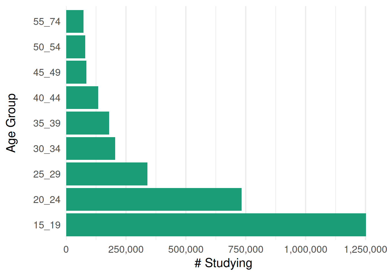
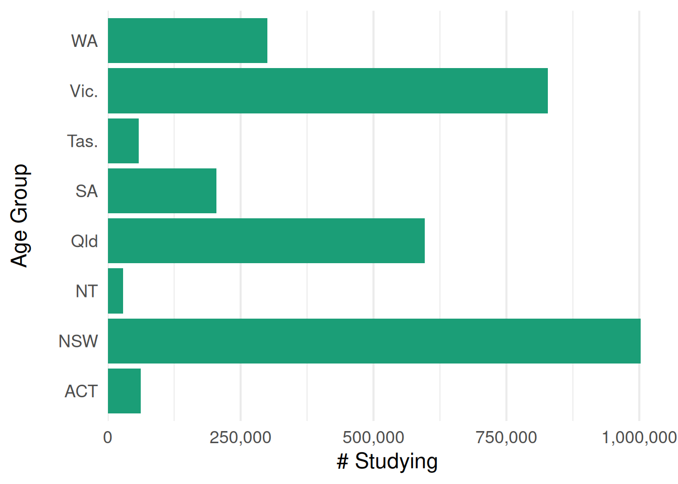
This is just one function, with two pretty different plots! The number studying for each age group, or for each state. The thing that changed is what variable goes on the y axis.

This can be tricky! Have you ever tried to write a function around dplyr or ggplot2? We will talk through how to solve this.

Now, the anatomy of a function.

2.2 The Anatomy of a function

Let’s answer a question with the data you read in last session. What percentage of 15 to 19 year olds are studying?

ed_2023 |>
  filter(age_group == "15_19") |>
  summarise(
    studying = sum(n_studying),
    people = sum(population)
  ) |>
  mutate(pct = round(studying / people * 100, 1))

# A tibble: 1 × 3
  studying people   pct
     <dbl>  <dbl> <dbl>
1    1252.  1542.  81.2

What if we want this to be for any age group?

Like I want to be able to write code that looks like this:

pct_studying(ed_2023, age = "25_29")

We can express this as a function:

pct_studying <- function(data, age = "25_29") {
  data_summary <- data |>
    filter(age_group == age) |>
    summarise(
      studying = sum(n_studying),
      people = sum(population)
    ) |>
    mutate(pct = round(studying / people * 100, 1))
  data_summary
}

pct_studying(ed_2023, age = "25_29")

# A tibble: 1 × 3
  studying people   pct
     <dbl>  <dbl> <dbl>
1     340.  1880.  18.1

Here are the key parts:

• The name is pct_studying. This is how you call it later.
• function() is what makes a function. The pct_studying <- bit just gives it a name, the same way you’d name any other object.
• The arguments are data and age. These are the parts that change between calls. You will also see them called formals, parameters, or args.
• The body is everything between the braces. This is the code that runs. When we use single braces like this, we are saying: Run multiple lines of code.
• The return value is whatever the body evaluates last, so here that is the one row table coming out of mutate().

The signature is the name plus the argument names: pct_studying(data, age).

The same parts, drawn out.

TipGoing deeper: other words for arguments

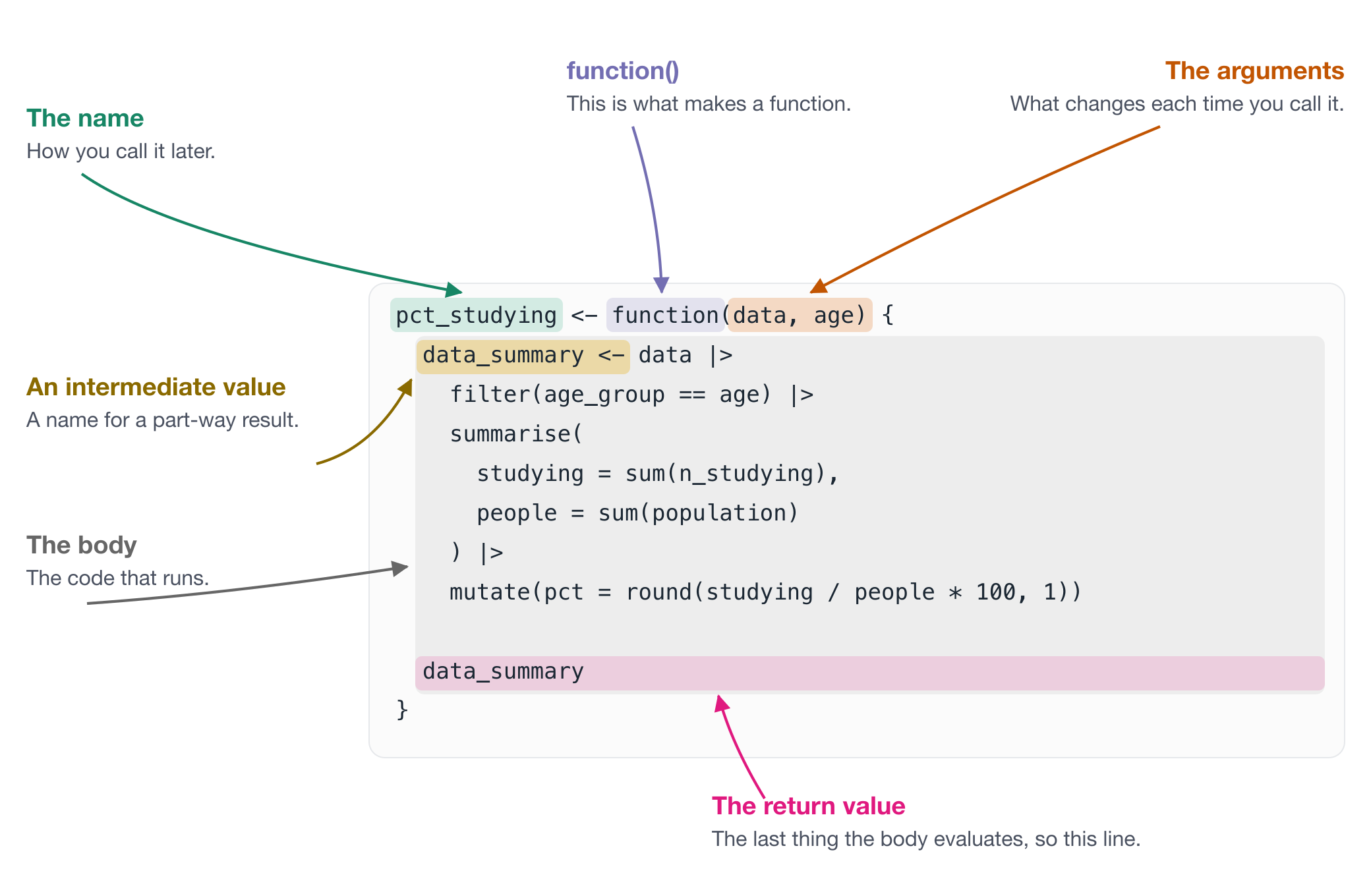
You will meet the same idea under several names. It is worth recognising all of them, so that a help page or an answer online does not throw you.

Arguments is the word I use, and the one the R documentation mostly uses.

Formals is R’s own internal word. formals() hands them back, with their defaults:

formals(pct_studying)

$data


$age
[1] "25_29"

Args is the abbreviation, and args() is a base R function that shows you the signature:

args(pct_studying)

function (data, age = "25_29") 
NULL

That NULL is not a mistake. args() gives you back a function with an empty body, and NULL is the body.

Parameters is the usual word in other languages, and it turns up in R writing too. Strictly, the parameter is the name in the definition and the argument is the value you hand over, so age is the parameter and "15_19" is the argument. Almost nobody holds that line, me included.

TipGoing deeper: when to write return()

R hands back whatever the body evaluates last, so most functions never need return() at all. The style most R code follows, and the one I follow, is this:

Only use return() to leave early.

Here is the case where I reach for it. If you ask pct_studying() for an age group that is not in the data, both sums come out as zero, and zero divided by zero is NaN. No error, no warning. An early return is one way to deal with that:

pct_studying_safe <- function(data, age = "25_29") {
  if (!age %in% data$age_group) {
    return(NULL)
  }

  data |>
    filter(age_group == age) |>
    summarise(
      studying = sum(n_studying),
      people = sum(population)
    ) |>
    mutate(pct = round(studying / people * 100, 1))
}

pct_studying_safe(tas_2023, age = "99_99")

NULL

The return(NULL) says “we are done here, there is nothing to work out”. Everything below it only runs when the age group is real.

A return() on the last line is different. It says nothing the code has not already said, and it is one more thing to read.

TipGoing deeper: functions are values

An argument can be a function. You hand it over without brackets, the same way you would hand over a number.

summarise_column <- function(values, fun) {
  fun(values)
}

summarise_column(values = education$n_studying, fun = mean)

[1] 42.54

summarise_column(values = education$n_studying, fun = max)

[1] 407.6

We are not calling mean there, we are passing it to the function. There are many powerful usecases of this. We will touch more on them later. For now, just know this kind of thing is possible.

NoteYour Turn: What do these return?

What do these functions return? Have a think about it, then run them and see!

my_summary <- function(values){
  list(
    min = min(values, na.rm = TRUE),
    median = median(values, na.rm = TRUE),
    mean = mean(values, na.rm = TRUE),
    max = max(values, na.rm = TRUE)
  )
}

# try running this with
# my_summary(ed_2023$n_studying)

my_summary2 <- function(values){
  summary_values <- list(
    min = min(values, na.rm = TRUE),
    q1 = quantile(values, probs = 0.25, na.rm = TRUE),
    median = median(values, na.rm = TRUE),
    mean = mean(values, na.rm = TRUE),
    q3 = quantile(values, probs = 0.75, na.rm = TRUE),
    max = max(values, na.rm = TRUE)
  )
}

# try running this with
# my_summary2(ed_2023$n_studying)

my_hist <- function(values){
  hist(values, main = "Histogram of values", breaks = "FD")
}
# try running this on
# ed_2023$n_studying

my_hist2 <- function(values){
  the_plot <- hist(values, main = "Histogram of values", breaks = "FD")
}
# try running this on
# ed_2023$n_studying

Takehomes

• The key parts of a function are: the name, the arguments, the body, the return value
• Arguments go by other names too: formals, parameters, args
• A function returns its last expression, so return() is for leaving early
• A function returns whatever its body evaluates last
• The signature is the name plus the argument names
• Knowing the words means you can search for them and ask about them

2.3 Default values

Functions can have default values. You’ve already seen one. Let’s explore defaults using plots.

tas_2023

# A tibble: 9 × 6
  state_territory age_group n_studying population prop_studying  year
  <chr>           <chr>          <dbl>      <dbl>         <dbl> <dbl>
1 Tas.            15_19           24.8       31.3       0.792    2023
2 Tas.            20_24            9.8       30.4       0.322    2023
3 Tas.            25_29            9         38.6       0.233    2023
4 Tas.            30_34            4.2       41.1       0.102    2023
5 Tas.            35_39            2         37.1       0.0539   2023
6 Tas.            40_44            3.5       34.2       0.102    2023
7 Tas.            45_49            2         32         0.0625   2023
8 Tas.            50_54            1.6       36.7       0.0436   2023
9 Tas.            55_74            1.3      143.        0.00907  2023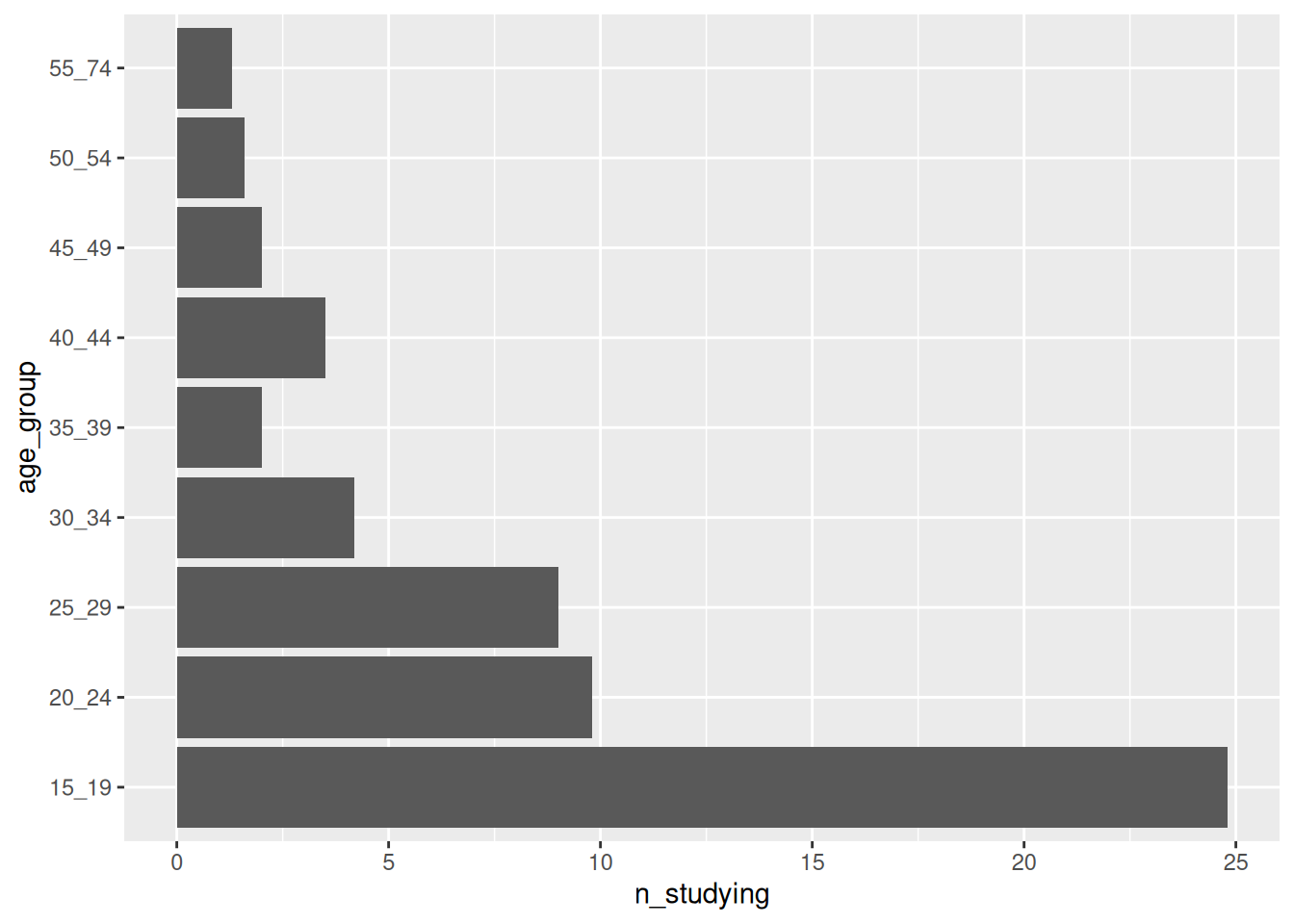

ggplot(tas_2023, aes(x = n_studying, y = age_group)) +
  geom_col()

Figure 2.3

Should we make that code above a function? My feeling is: probably not.

My reasons:

• ggplot expressed itself well
• I’m unlikely to run the same thing again
• There isn’t that much code - so I can understand what it is expressing easily

We don’t need to always “make everything a function”.

Like, I’m not sure if we would get out of a function like so:

plot_study_by_age <- function(data, state){
  ggplot(data, aes(x = n_studying, y = age_group)) +
  geom_col() + 
    labs(title = state)
}

plot_study_by_age(tas_2023, state = "Tas.")

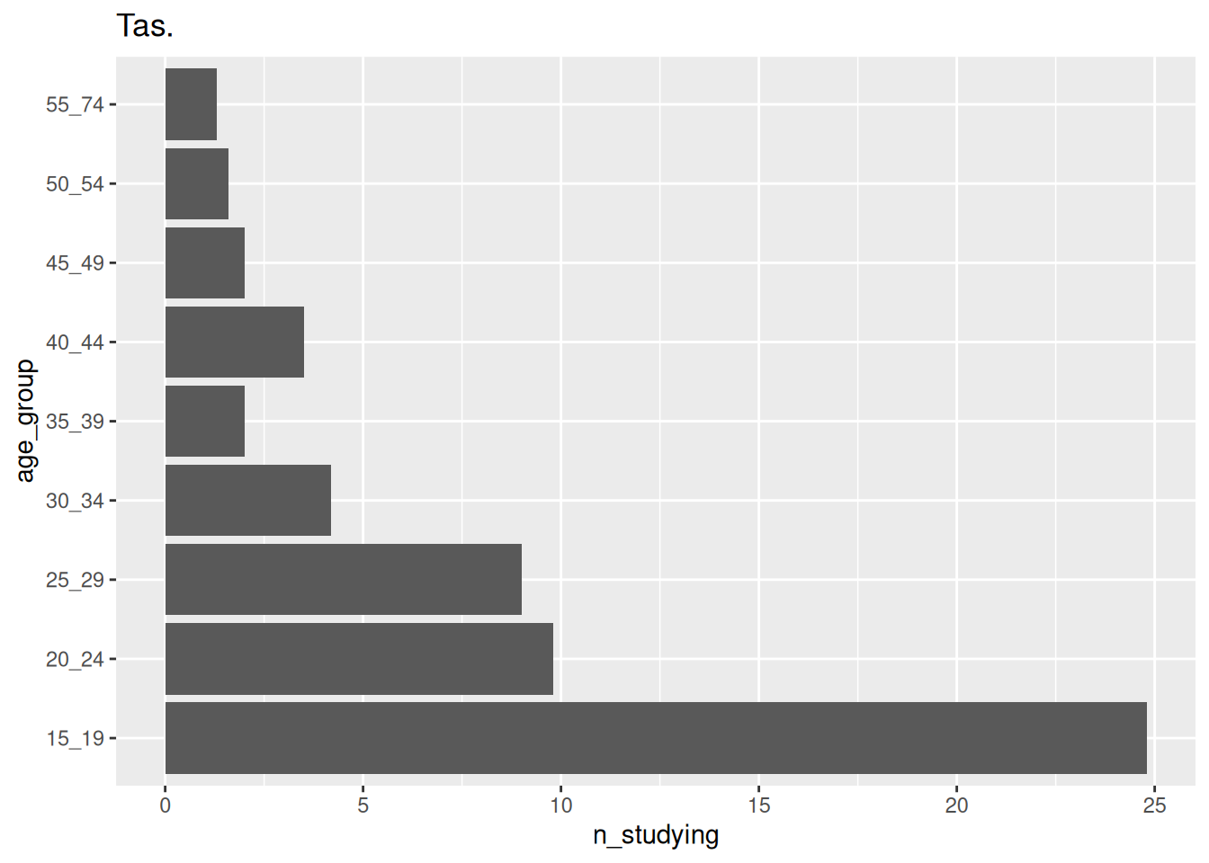
But what might tip the balance towards creating a function is if we were really tinkering with a lot of the plotting options. If this plot now does the following:

• The axis labels are column names
• The x axis should be in increments of 1,000
• It could use a title, and a colour that is not battleship grey
• The left axis of the bars should be aligned

ggplot(tas_2023, aes(x = n_studying, y = age_group)) +
    geom_col(fill = "#1B9E77") +
    labs(x = "# Studying", y = "Age Group") +
    theme_minimal(base_size = 16) +
    theme_sub_panel(grid.major.y = element_blank()) +
    scale_x_continuous(labels = label_number(scale = 1000, big.mark = ","),
                       expand = expansion(mult = c(0, 0.05)), limits = c(0,NA)) +
    theme_sub_axis_y(title = element_text(margin = margin(r = 20)))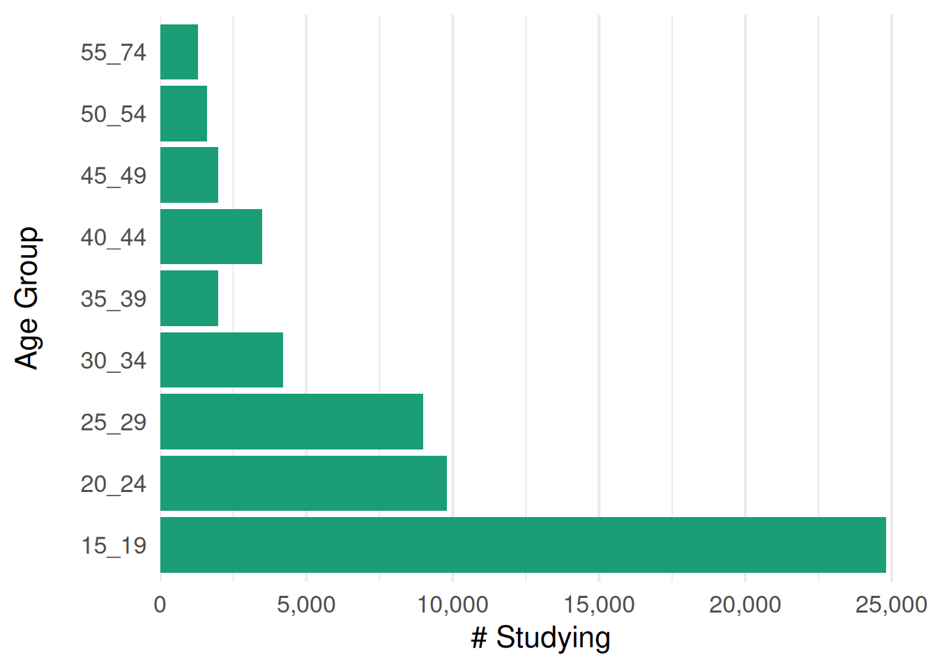

Let’s write this as a function - we want to change the data, but have everything else the same

plot_study_by_age <- function(data, state) {
  ggplot(data, aes(x = n_studying, y = age_group)) +
    geom_col(fill = "#1B9E77") +
    labs(x = "# Studying", y = "Age Group") +
    theme_minimal(base_size = 16) +
    theme_sub_panel(grid.major.y = element_blank()) +
    scale_x_continuous(labels = label_number(scale = 1000, big.mark = ","),
                       expand = expansion(mult = c(0, 0.05)), limits = c(0,NA)) +
    theme_sub_axis_y(title = element_text(margin = margin(r = 20)))
}

plot_study_by_age(tas_2023, state = "Tas.")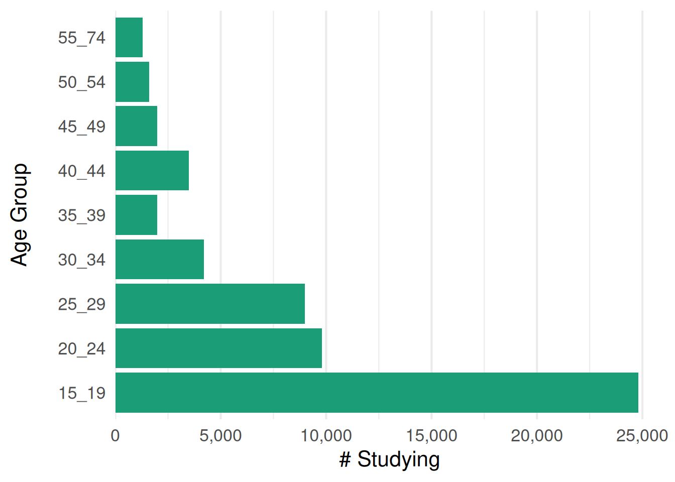

Now the fiddly decisions live in one place. But look at how you have to call it.

plot_study_by_age(tas_2023, state = "Tas.")

An argument can have a default, which is the value it takes when you do not specify one.

plot_study_by_age <- function(data, state = "Tas.") {
  ggplot(tas_2023, aes(x = n_studying, y = age_group)) +
    geom_col(fill = "#1B9E77") +
    theme_minimal(base_size = 16) +
    theme_sub_panel(grid.major.y = element_blank()) +
    scale_x_continuous(labels = label_number(scale = 1000, big.mark = ","),
                       expand = expansion(mult = c(0, 0.05)), limits = c(0,NA)) +
    theme_sub_axis_y(title = element_text(margin = margin(r = 20))) +
    labs(
      x = "Studying",
      y = "Age group",
      title = "Proportion of people studying, by age group",
      subtitle = state
    )
}

The default here is “Tas.”

plot_study_by_age(tas_2023)

Figure 2.4

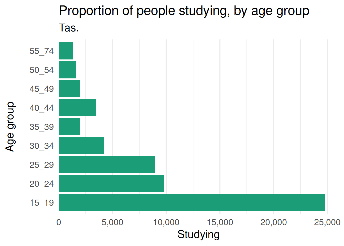
The subtitle says “Tas.” and I never typed it, because the default was specified.

We could change that to:

plot_study_by_age(tas_2023, state = "Tasmania, 2023")

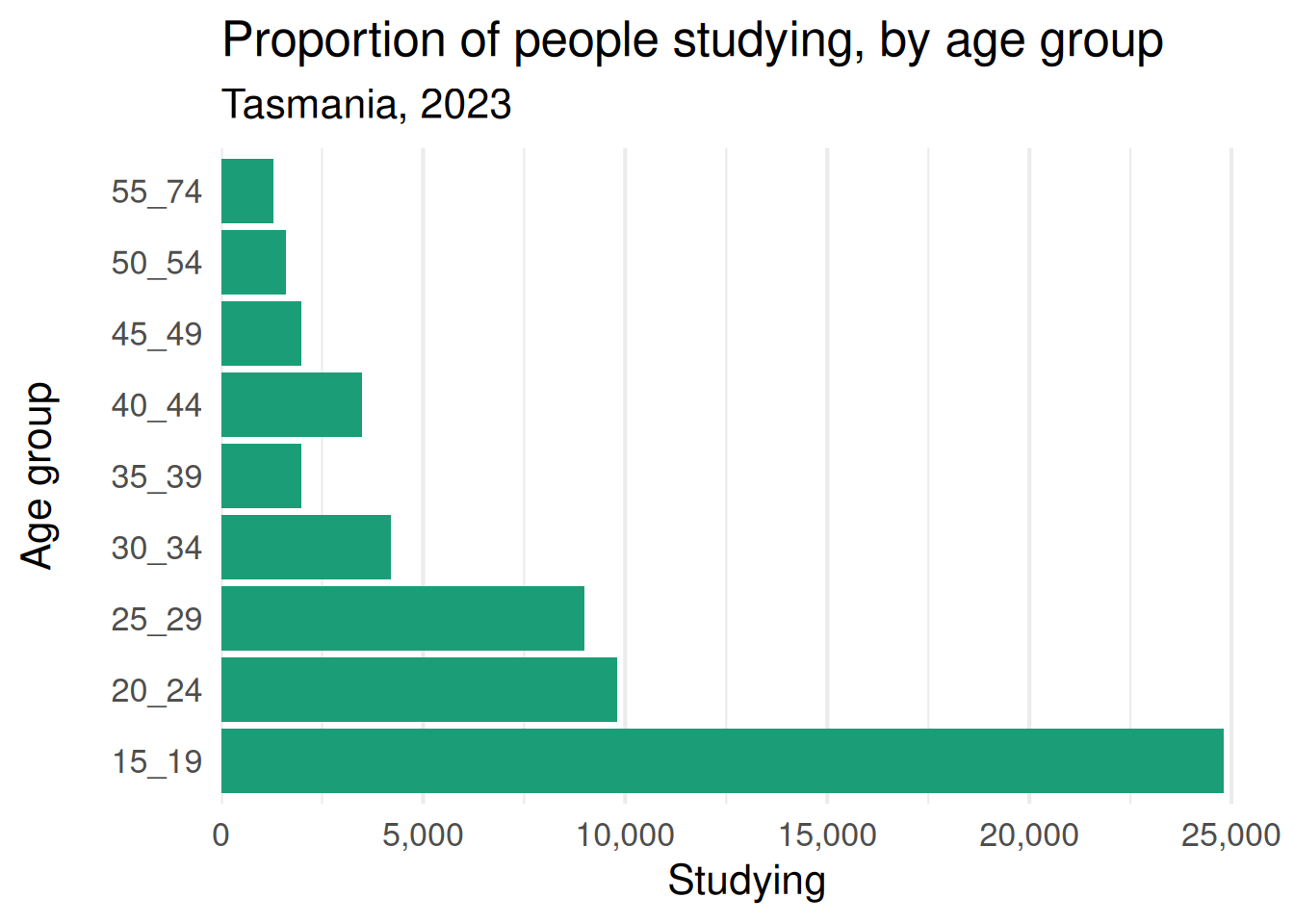
That’s what defaults are for. They make the common case easy without taking away control in the uncommon one.

TipGoing deeper: defaults that use the other arguments

A default does not have to be a fixed value. It can be worked out from the other arguments, because defaults are evaluated inside the function, after the caller’s values have arrived.

plot_study_titled <- function(
  data,
  state,
  title = glue("Proportion studying in {state}")
) {
  ggplot(data, aes(x = n_studying, y = age_group)) +
    geom_col(fill = "#1B9E77") +
    scale_x_continuous(labels = label_number(scale = 1000, big.mark = ","),
                       expand = expansion(mult = c(0, 0.05)), limits = c(0,NA)) +
    theme_sub_axis_y(title = element_text(margin = margin(r = 20))) +
    labs(x = "Studying", y = "Age group", title = title) +
    theme_minimal(base_size = 16)
}

plot_study_titled(tas_2023, state = "Tas.")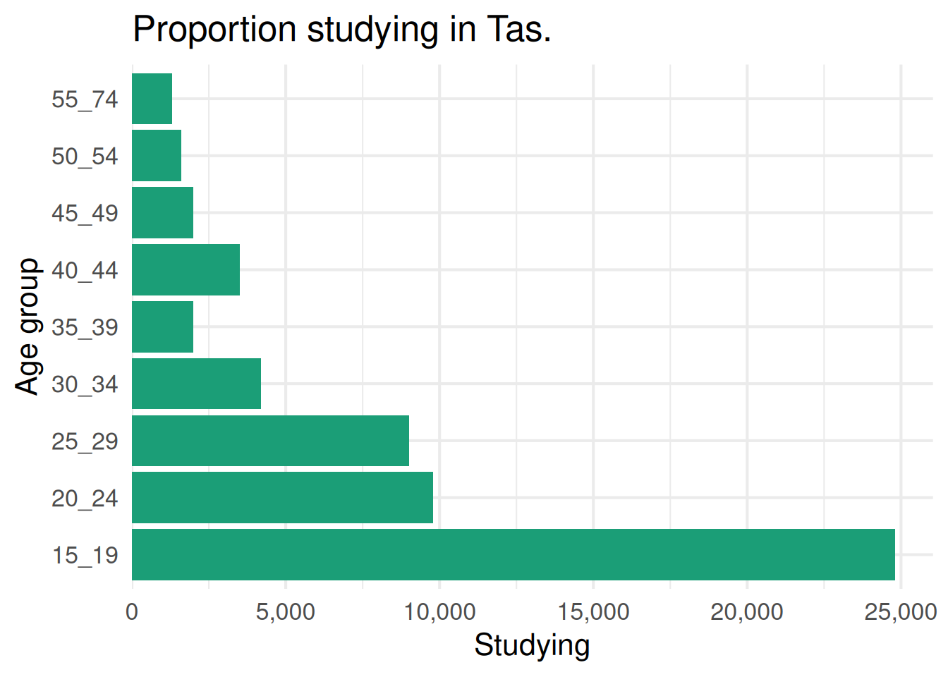

Figure 2.5

The title writes itself from state, so the common case needs one argument instead of two.

The catch is that you can now pass two things that disagree, and nothing stops you:

plot_study_titled(tas_2023, state = "Tas.", title = "Victoria")

Figure 2.6

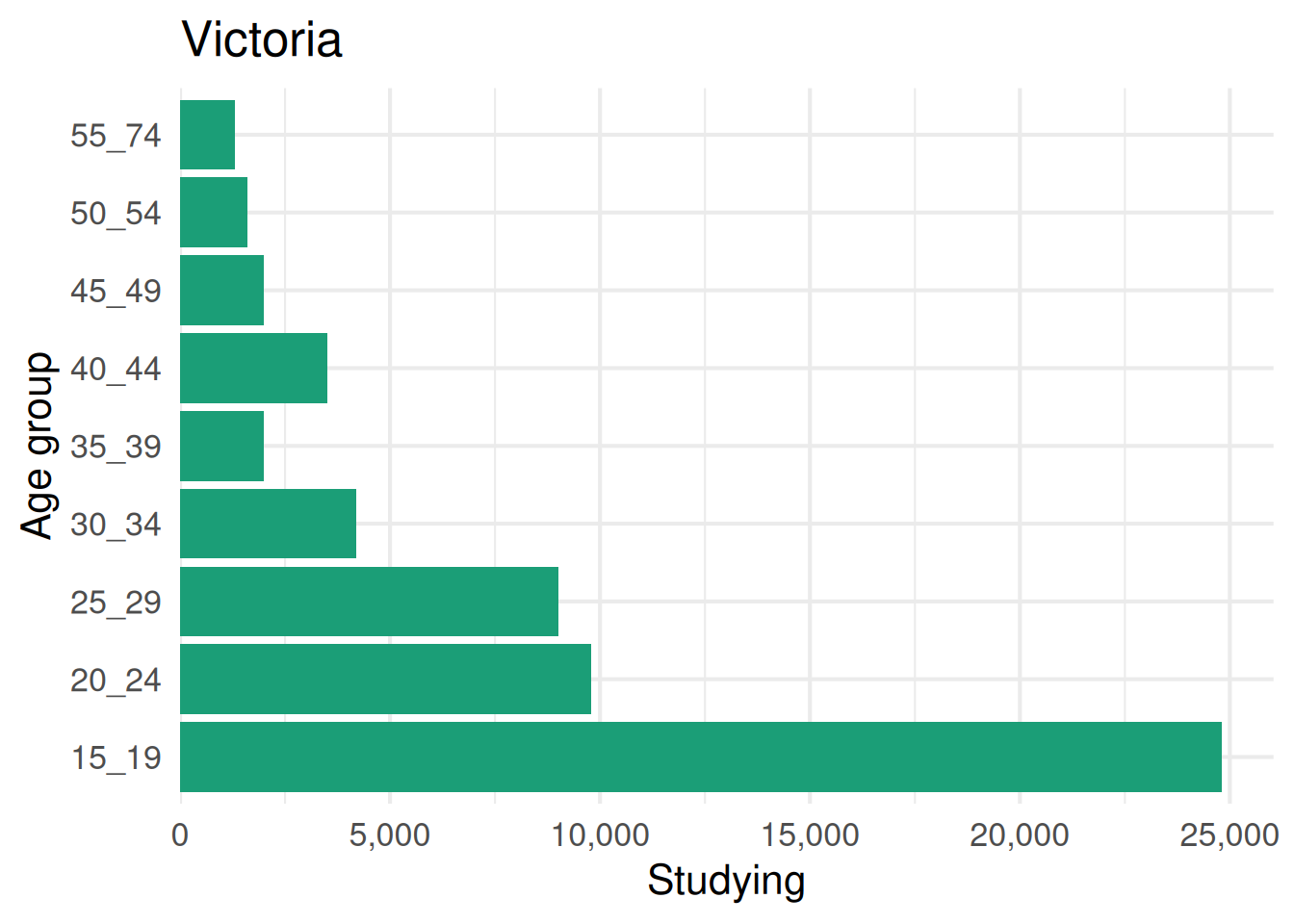
Two arguments that have to agree with each other are a bug waiting to happen. Here it is only a wrong title. When it is a filter and a label, it is a wrong answer with a confident heading on it.

NoteYour Turn

Setup code

library(countdown)
library(dplyr)
library(readr)
library(ggplot2)
library(glue)
library(here)
library(scales)
education_path <- function(year) {
  here(glue("data/tidy/education_{year}.csv"))
}

year_from_path <- function(path) {
  basename(path) |>
    parse_number()
}

read_education <- function(year) {
  files <- education_path(year)
  education_raw <- read_csv(files, id = "path")

  education_raw |>
    mutate(year = year_from_path(path)) |>
    select(-path)
}

education <- read_education(2014:2023)

ed_2023 <- education |>
  filter(year == 2023)

tas_2023 <- education |>
  filter(year == 2023, state_territory == "Tas.")

plot_study_by <- function(data, y) {
  ggplot(data, aes(x = n_studying, y = {{ y }})) +
    geom_col(fill = "#1B9E77") +
    scale_x_continuous(labels = label_number(scale = 1000, big.mark = ","),
                       expand = expansion(mult = c(0, 0.05)), limits = c(0,NA)) +
    labs(x = "# Studying", y = "Age Group") +
    theme_minimal(base_size = 16) +
    theme_sub_panel(grid.major.y = element_blank()) +
    theme_sub_axis_y(title = element_text(margin = margin(r = 20)))
}

pct_studying <- function(data, age = "25_29") {
  data_summary <- data |>
    filter(age_group == age) |>
    summarise(
      studying = sum(n_studying),
      people = sum(population)
    ) |>
    mutate(pct = round(studying / people * 100, 1))
  data_summary
}

pct_studying(ed_2023, age = "25_29")

1. Call pct_studying(tas_2023) with no age at all. Which age group did you get?
2. Ask for an age group that is not in the data, like "99_99". You should get a number, not an error. What is it?

Answer

pct_studying(tas_2023)

# A tibble: 1 × 3
  studying people   pct
     <dbl>  <dbl> <dbl>
1        9   38.6  23.3

pct_studying(tas_2023, age = "99_99")

# A tibble: 1 × 3
  studying people   pct
     <dbl>  <dbl> <dbl>
1        0      0   NaN

The first is the default, "25_29", which is what you get when you do not say.

The second is the interesting one. No rows match "99_99", so both sums are zero, and zero divided by zero is NaN. No error and no warning.

Takehomes

• A default is the value an argument takes when the caller does not supply one
• Defaults can be worked out from the other arguments
• Give the common case a default, and let people override it
• Two arguments that must agree with each other are a bug waiting to happen

2.4 Arguments by position and by order

Arguments can be given:

• By name
• By position

By name, using name = value:

pct_studying(data = tas_2023, age = "15_19")

# A tibble: 1 × 3
  studying people   pct
     <dbl>  <dbl> <dbl>
1     24.8   31.3  79.2

By position, in the order the definition lists them:

pct_studying(tas_2023, "15_19")

# A tibble: 1 × 3
  studying people   pct
     <dbl>  <dbl> <dbl>
1     24.8   31.3  79.2

Once they’re named, the order/position doesn’t matter:

pct_studying(age = "15_19", data = tas_2023)

# A tibble: 1 × 3
  studying people   pct
     <dbl>  <dbl> <dbl>
1     24.8   31.3  79.2

pct_studying(data = tas_2023, age = "15_19")

# A tibble: 1 × 3
  studying people   pct
     <dbl>  <dbl> <dbl>
1     24.8   31.3  79.2

And you can mix the two:

pct_studying(tas_2023, age = "15_19")

# A tibble: 1 × 3
  studying people   pct
     <dbl>  <dbl> <dbl>
1     24.8   31.3  79.2

All four give 24.8, 31.3, 79.2. What differs is how much you need to already know in order to read the line.

Naming arguments costs a few keystrokes and buys a line that reads on its own.

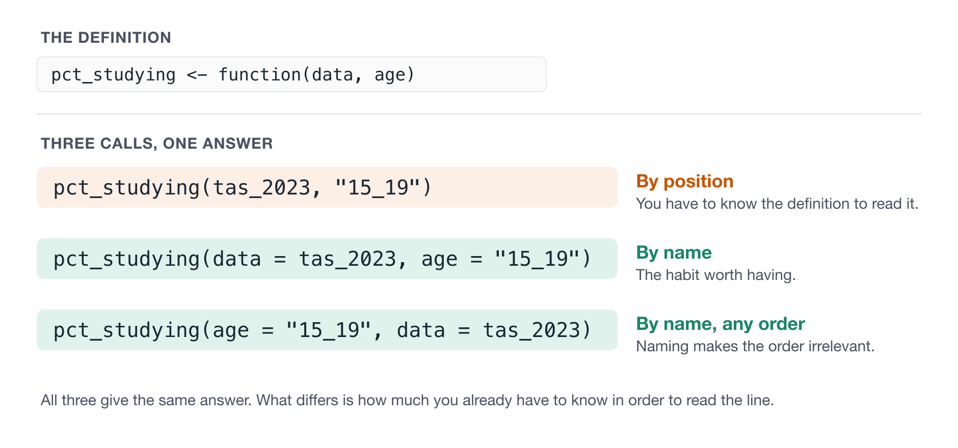
pct_studying(tas_2023, "15_19") needs you to remember what the second slot is for. pct_studying(tas_2023, age = "15_19") tells you.

I leave the first argument positional, because it’s nearly always the data and nobody is confused by it. Everything after that, I name.

NoteYour Turn

Setup code

library(countdown)
library(dplyr)
library(readr)
library(ggplot2)
library(glue)
library(here)
library(scales)
education_path <- function(year) {
  here(glue("data/tidy/education_{year}.csv"))
}

year_from_path <- function(path) {
  basename(path) |>
    parse_number()
}

read_education <- function(year) {
  files <- education_path(year)
  education_raw <- read_csv(files, id = "path")

  education_raw |>
    mutate(year = year_from_path(path)) |>
    select(-path)
}

education <- read_education(2014:2023)

ed_2023 <- education |>
  filter(year == 2023)

tas_2023 <- education |>
  filter(year == 2023, state_territory == "Tas.")

plot_study_by <- function(data, y) {
  ggplot(data, aes(x = n_studying, y = {{ y }})) +
    geom_col(fill = "#1B9E77") +
    scale_x_continuous(labels = label_number(scale = 1000, big.mark = ","),
                       expand = expansion(mult = c(0, 0.05)), limits = c(0,NA)) +
    labs(x = "# Studying", y = "Age Group") +
    theme_minimal(base_size = 16) +
    theme_sub_panel(grid.major.y = element_blank()) +
    theme_sub_axis_y(title = element_text(margin = margin(r = 20)))
}

pct_studying <- function(data, age = "25_29") {
  data_summary <- data |>
    filter(age_group == age) |>
    summarise(
      studying = sum(n_studying),
      people = sum(population)
    ) |>
    mutate(pct = round(studying / people * 100, 1))
  data_summary
}

pct_studying(ed_2023, age = "25_29")

1. Call pct_studying() on tas_2023 for 20 to 24 year olds, naming both arguments.
2. Swap the order of those two named arguments. Does it still work?
3. Now guess before you run it: does pct_studying("20_24", data = tas_2023) work?

Answer

pct_studying(data = tas_2023, age = "20_24")

# A tibble: 1 × 3
  studying people   pct
     <dbl>  <dbl> <dbl>
1      9.8   30.4  32.2

pct_studying(age = "20_24", data = tas_2023)

# A tibble: 1 × 3
  studying people   pct
     <dbl>  <dbl> <dbl>
1      9.8   30.4  32.2

pct_studying("20_24", data = tas_2023)

# A tibble: 1 × 3
  studying people   pct
     <dbl>  <dbl> <dbl>
1      9.8   30.4  32.2

All three give the same answer. The third one works because data was named, so the only slot left for "20_24" is age.

I would not write that third one. But it is worth knowing that R takes the named arguments first, then pours whatever is left into the gaps in order.

Takehomes

• You can pass arguments by position or by name
• Naming them means the order does not matter
• Leave the first one positional, name the rest
• A named argument saves your reader a trip to the definition

2.5 Making a function work on any column

plot_study_by_age() always plots age_group.

If I want the same plot broken down by state instead?

I could copy the whole function and change one word, which is where we came in.

NoteYour Turn: plotting functions

How would you change plot_study_by_age() to be plotted by state, or age group, or some other variable?

plot_study_by_age <- function(data, state = "Tas.") {
  ggplot(tas_2023, aes(x = n_studying, y = age_group)) +
    geom_col(fill = "#1B9E77") +
    theme_minimal(base_size = 16) +
    theme_sub_panel(grid.major.y = element_blank()) +
    scale_x_continuous(labels = label_number(scale = 1000, big.mark = ","),
                       expand = expansion(mult = c(0, 0.05)), limits = c(0,NA)) +
    theme_sub_axis_y(title = element_text(margin = margin(r = 20))) +
    labs(
      x = "Studying",
      y = "Age group",
      title = "Proportion of people studying, by age group",
      subtitle = state
    )
}

So let’s try the obvious thing and pass the column as an argument.

plot_study_by <- function(data, y) {
  ggplot(data, aes(x = n_studying, y = y)) +
    geom_col()
}

plot_study_by(tas_2023, y = age_group)

Error in `geom_col()`:
! Problem while computing aesthetics.
ℹ Error occurred in the 1st layer.
Caused by error:
! object 'age_group' not found

You should get an error. That isn’t you doing it wrong, and it’s the wall that stops a lot of people writing functions around dplyr and ggplot2.

The problem is that age_group is not a value sitting in your workspace. It’s a column name, and it only means anything once you’re inside the data. R tries to look it up before it ever gets there.

The fix is to wrap the argument in two sets of braces, which people say out loud as curly curly.

plot_study_by <- function(data, y) {
  ggplot(data, aes(x = n_studying, y = {{ y }})) +
    geom_col(fill = "#1B9E77") +
    scale_x_continuous(labels = label_number(scale = 1000, big.mark = ",")) +
    labs(x = "# Studying", y = NULL) +
    theme_minimal(base_size = 12)
}

plot_study_by(tas_2023, y = age_group)

Figure 2.7

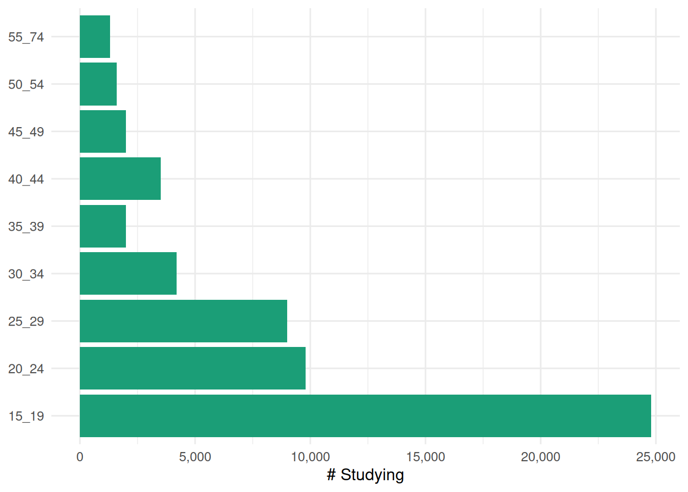
{{ y }} means “do not look this up yet, pass it through to the data”. That’s all you need to know today, and it works the same way in dplyr.

Some terms to be aware of, and discuss, if time:

• standard evaluation vs Non-standard evaluation
• quasiquotation - quoting/unquoting

TipGoing deeper: why curly braces?

The braces are a deliberate echo of glue().

In glue("education_{year}.csv") last session, { } meant “look this up and put the value here”. In {{ y }} they mean much the same thing. What gets put there is the column the caller named, and it gets looked up inside the data rather than in your workspace.

So if glue() made sense last session, curly curly is the same instinct with one more layer of braces.

And now the same plotting function does a different job entirely:

education |>
  filter(year == 2023, age_group == "15_19") |>
  plot_study_by(y = state_territory)

Figure 2.8

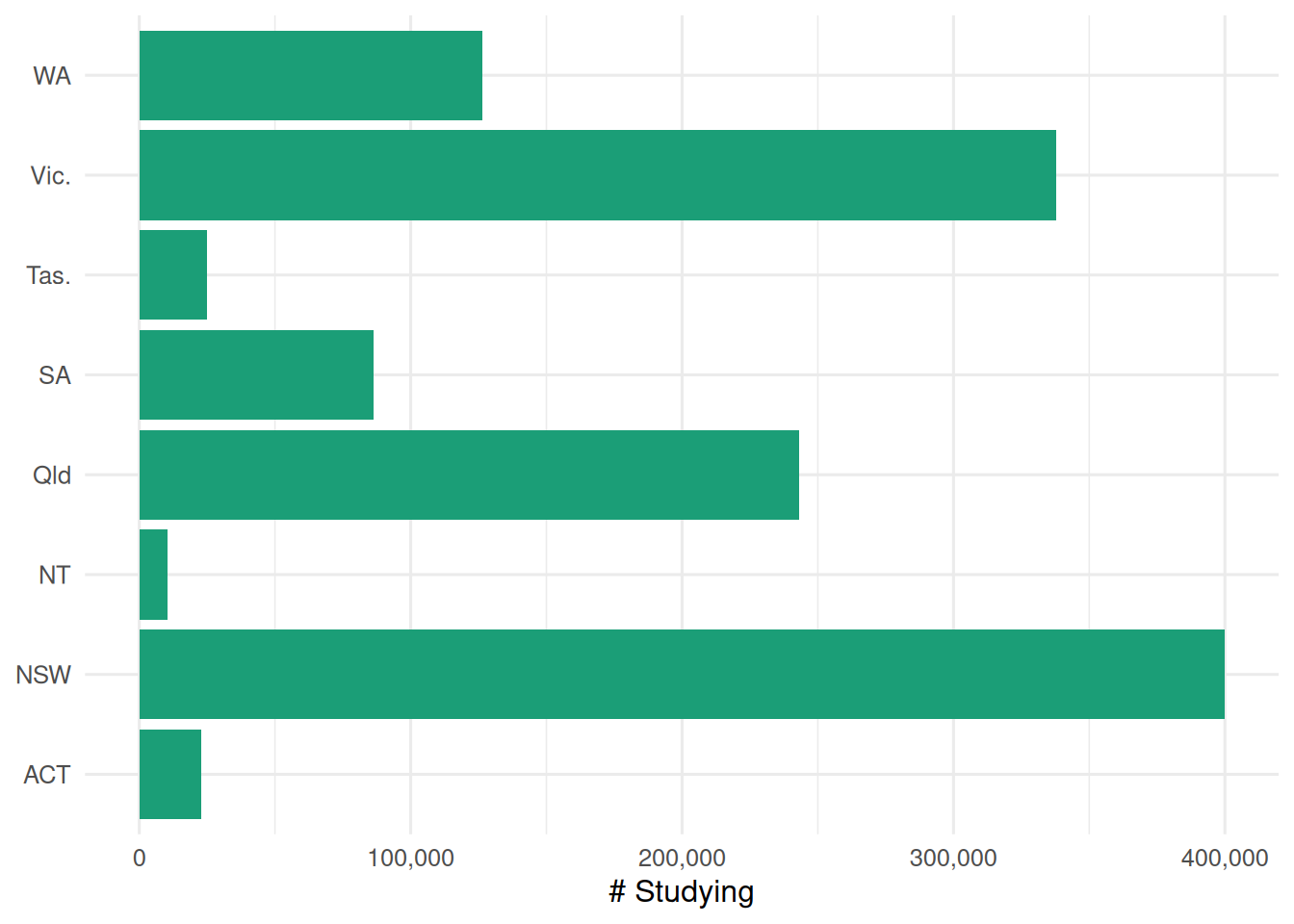
Notice I renamed it. plot_study_by_age() was true when it only did age groups, but now it is more general.

It is normal to iterate on a plot name. The first name you pick is rarely the one you keep, and renaming is part of writing a function rather than a sign you’ve got it wrong.

You can read more about curly curly at:

• My blog post: Curly Curly: How to pass bare variable arguments to things?
• The dplyr documentation: Programming with dplyr
• ggplot2 docs: ggplot2 in packages

NoteYour Turn

Setup code

library(countdown)
library(dplyr)
library(readr)
library(ggplot2)
library(glue)
library(here)
library(scales)
education_path <- function(year) {
  here(glue("data/tidy/education_{year}.csv"))
}

year_from_path <- function(path) {
  basename(path) |>
    parse_number()
}

read_education <- function(year) {
  files <- education_path(year)
  education_raw <- read_csv(files, id = "path")

  education_raw |>
    mutate(year = year_from_path(path)) |>
    select(-path)
}

education <- read_education(2014:2023)

ed_2023 <- education |>
  filter(year == 2023)

tas_2023 <- education |>
  filter(year == 2023, state_territory == "Tas.")

plot_study_by <- function(data, y) {
  ggplot(data, aes(x = n_studying, y = {{ y }})) +
    geom_col(fill = "#1B9E77") +
    scale_x_continuous(labels = label_number(scale = 1000, big.mark = ","),
                       expand = expansion(mult = c(0, 0.05)), limits = c(0,NA)) +
    labs(x = "# Studying", y = "Age Group") +
    theme_minimal(base_size = 16) +
    theme_sub_panel(grid.major.y = element_blank()) +
    theme_sub_axis_y(title = element_text(margin = margin(r = 20)))
}

1. Use plot_study_by() on the ACT in 2023, broken down by age_group.
2. Write median_by() yourself, on the same shape as mean_by(), and use it to get the median by age_group.
3. Give plot_study_by() a default for y, so that plot_study_by(tas_2023) works with no second argument.

Answer

act_2023 <- education |> filter(year == 2023, state_territory == "ACT")
plot_study_by(act_2023, y = age_group)

median_by <- function(data, group) {
  data |>
    group_by({{ group }}) |>
    summarise(median_prop = round(median(n_studying), 3), .groups = "drop")
}

median_by(filter(education, year == 2023), group = age_group)

The only thing that changed from mean_by() is the summary function. {{ }} does the same job either way.

For step 3, the default goes in the signature the same as any other:

plot_study_by <- function(data, y = age_group) {
  ggplot(data, aes(x = n_studying, y = {{ y }})) +
    geom_col(fill = "#1B9E77")
}

Takehomes

• Column names are not values, so passing them straight in does not work
• Wrap the argument in {{ }} to pass a column through to dplyr or ggplot2
• One function then covers every column instead of one
• When a function outgrows its name, rename it

2.6 Naming things

Is hard!

A function does something, it is us expressing out intention! So take a moment to think about that when you give something a name.

There is a process, it might take iteration:

myfun()            # what?
study_plot()       # better, but what does it do with it?
plot_study_by()    # now I do not have to read the body

A template I like is: verb_noun().

• the thing you do
• the thing it happens on

Let’s discuss.

Takehomes

• verb_noun() is a good default shape
• Name for the question, not the method
• The names inside the body matter as much as the one outside
• If you cannot name it, you probably have two functions

Summary

1. The parts are name, arguments, body, return value. The signature is the name plus the argument names.
2. Defaults make the common case easy. They can be worked out from the other arguments.
3. Name your arguments when you call something, except the first.
4. {{ }} passes a column name through to dplyr and ggplot2.
5. Renaming is part of writing. When a function outgrows its name, change it.

Links

• Curly Curly: How to pass bare variable arguments to things?
• Programming with dplyr
• ggplot2 in packages